A cycling map of Baltimore's neighborhoods
There are 279 neighborhoods in Baltimore. These neighborhoods are often used as identifying locations in news stories or event announcements, and it’s a bit of a mark of a local to know them. In addition, Wandrer makes each of them into an achievement, awarding points as you complete all their streets. Yet their sheer number makes it very difficult to track them all. I wanted to keep track of them in order to earn my “local” badge and get to know the city a bit better. For that, it’s hard to beat a physical map.
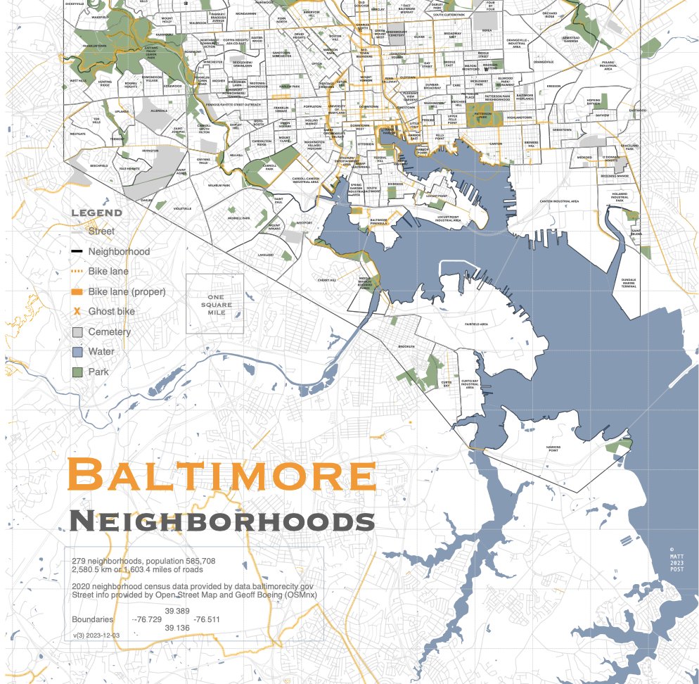
The city itself provides an official neighborhoods map, but it is ugly:
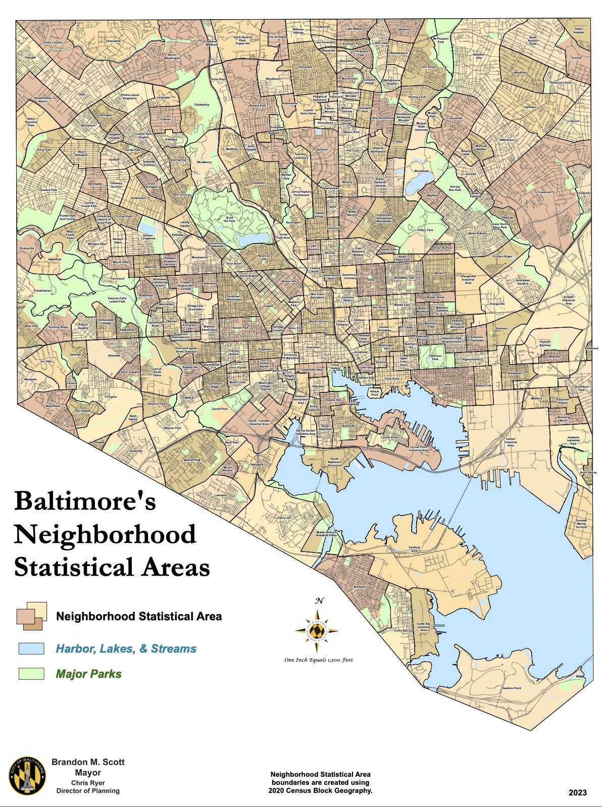
So I decided to create my own.
Background on building custom maps
It took me quite some time to figure out the lay of the land on custom map building. Here is a bit of what I learned.
The scalar approach
There are at least two ways to create maps. The first is to download tiles from a service like Mapbox or Open Street Map. These pre-rendered images have been curated by a team of cartographers, who have done things like choose colors, line widths, and, crucially, placed labels for streets and points of interest. To use tiles, you need the latitude and longitude of the region, as well as the zoom level. This article provides a nice overview of how to use them, and in particular points to this tool for obtaining this information for different regions (another nice tool is https://overpass-turbo.eu/). Here is an exmaple of Druid Hill Park in Baltimore.
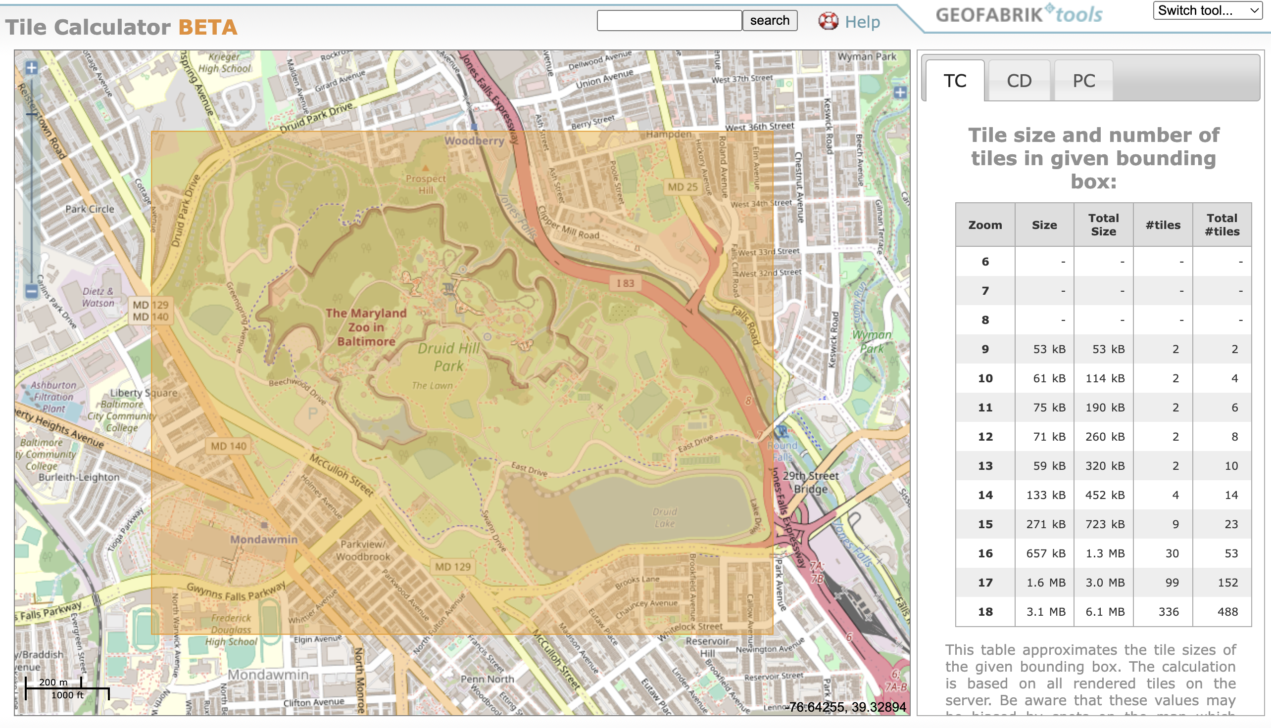
The disadvantage of the tile approach is that you’re stuck with the features that the curators found interesting or useful. Their use cases were different from mine. Fortunately there is another approach.
The vector approach
The second way is to download the raw data and render it yourself. Open Street Map (OSM)1 is a crowd-sourced map of the world. It is a bit like Wikipedia, but for maps. You—yes, you—can go to Open Street Map and use its rich tools to create roads and structures and, additionally, to tag these features with a rich taxonomy of metadata. The data is all recorded as polygons and lines, which means that they can be natively plotted at any resolution. This is the vector approach.
The rich annotations in Open Street Map allow you to download exactly and only the data you want; you then have to do the rendering yourself.
Fortunately there are a number of tools that make this easy.
Chief among them is the OSMnx python module, which provides a Python library for querying and downloading OSM data and converting it into GeoPandas data frames, which handle projection of latitude/longitude data to a 2d coordinate system.
Plotting can then be done with Python’s matplotlib.
This approach is not without its disadvantages. The main one is that placing street labels turns out to be quite difficult; with tiles, this is done for you. Fortunately, I didn’t need street labels, but only the neighborhood-level information. A second, deeper problem is that you now have an art project on your hands. I don’t have general solutions to that other than ad nauseum iteration.
The Baltimore map
OSM maintains polygons for geopolitical entities at different administrative levels (tag: admin_level=*), ranging from 1 to 10.
Level 1 is the complete earth.
Level 2 is for countries, and in the USA, level 6 for large cities that also function as state counties or equivalents, and level 8 for smaller cities.
Level 10 is reserved for neighborhoods and homeowners’ associations, and are in fact somewhat rare.
Seattle, for example, has no neighborhood-level information, and neither does Grand Rapids, Michigan.
St. Louis, Missouri, on the other hand, has a very rich set of neighborhoods, as does Baltimore.
The neighborhood information on Baltimore is, however, incomplete. Fortunately, the city of Baltimore’s excellent Open Data portal provides a GeoJSON file (click on Download) with the boundaries of all 279 of its neighborhoods.2 There is also a nice interactive map that shows the neighborhoods as if they were a big tiled puzzle.
The grid above shows my first two attempts. For the first version, to get the street data, I used a version of the following code:
import osmnx as ox
import geopandas as gpd
import matplotlib.pyplot as plt

common_crs = "EPSG:4326"

# Load the neighborhoods data from the city of Baltimore's file
gdf_neighborhoods = gpd.read_file("data/Baltimore.geojson")
gdf_neighborhoods.crs = common_crs

# Using a network type of "all_private" will get all the alleys etc
# It also makes the boundaries with water a lot fuzzier since they
# are overlaid.
west, south, east, north = gdf_neighborhoods.total_bounds
G = ox.graph_from_bbox(north, south, east, west, network_type="drive", retain_all=True)

# Convert to a GeoDataFrame and project to a common CRS
gdf_streets = ox.graph_to_gdfs(G, nodes=False, edges=True, node_geometry=False, fill_edge_geometry=True)
gdf_streets = gdf_streets.to_crs(common_crs)
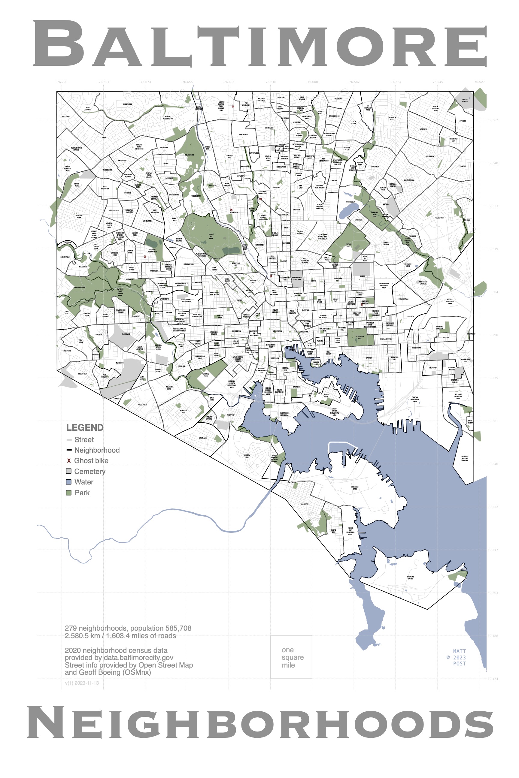
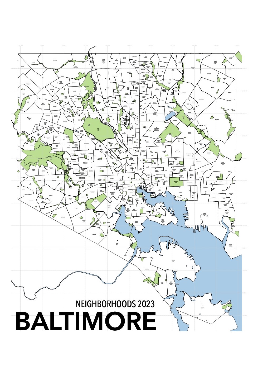
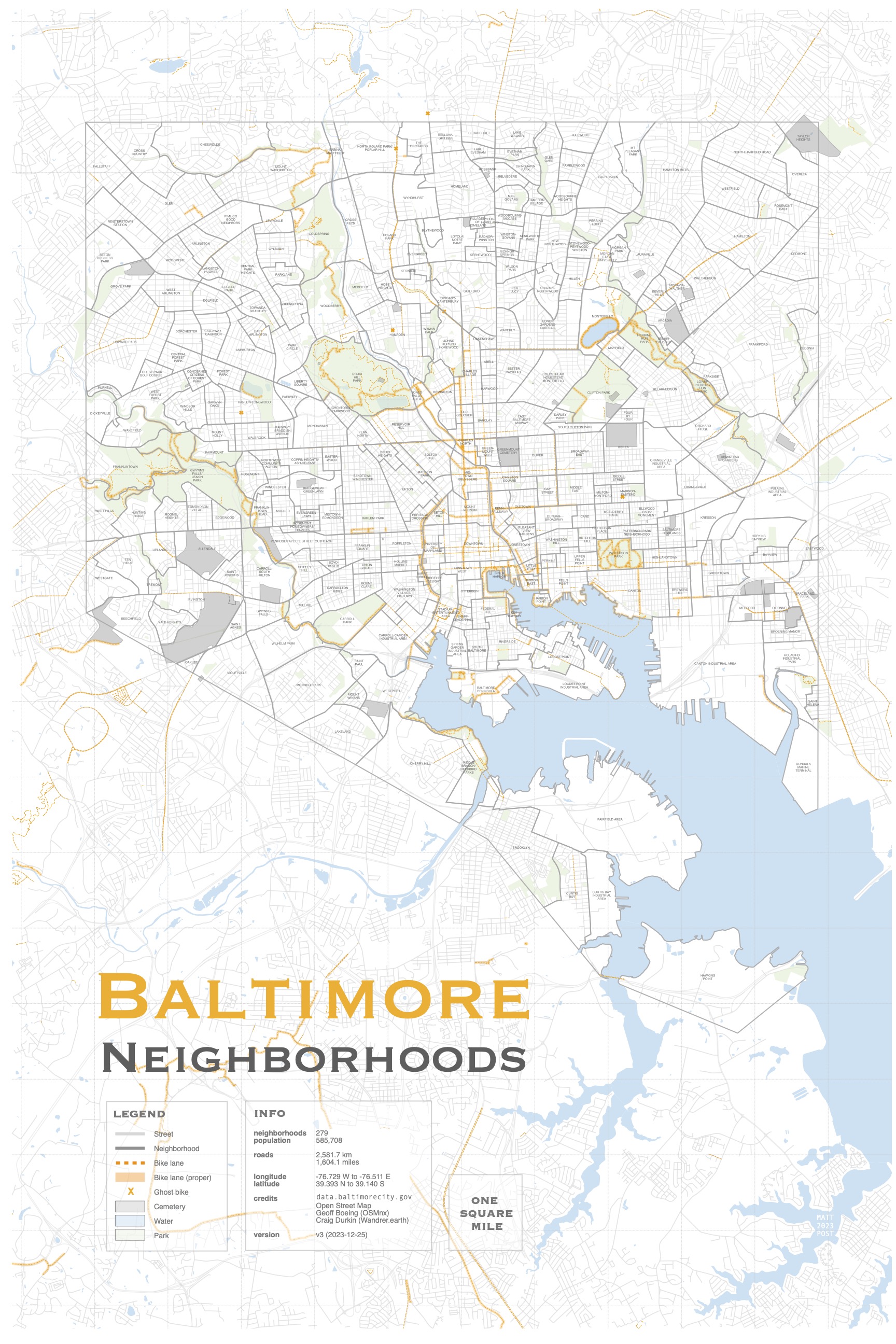
My goal was to print this at 2’ x 3’, so there was a bunch of header and footer space to fill. I originally filled this with the map title (v1), but soon came to hate this look, since it dominated the space. In v2, I adopted the city’s approach of fitting the map title and information in the SW quadrant, where there is plenty of space.
The deadspace on the top and bottom remained a problem. It took a while, but I realized that my favorite map feature was the Patapsco River extending out of the city boundaries. This led to an idea to plot all streets, parks, and other data to bleed to the edge of the map. A snippet of this can be seen in v3 of the map.
To make this work within my frame, I had to extend the bleed to my 1.5 ratio. The following code determines the vertical bounding box based on the city width (since I know that Baltimore is taller than it is wide).
# Some definitions. A mile of longitude at Baltimore's average latitude is about 0.018.
one_mile_lat = 0.01446
def one_mile_lon(lat):
    return 0.0144927536231884 * math.cos(lat * math.pi / 180)

# Add some margin to the map boundaries
west -= one_mile_lon
east += one_mile_lon

# For the north/south adjustments, we need to take into account the
# curvature of the earth. Here we find how much we need to add to the Y
# access, using the mid-latitude point as an approximation.
# return the distance between two longitude coordinates at a given latitude
def lon_distance(lon1, lon2, lat):
    return (lon2 - lon1) * math.cos(lat * math.pi / 180)

# Find the vertical distance we need to add in order to get a 1.5 ratio
compensation = 1.5 * lon_distance(west, east, (north + south) / 2) - (north - south)
# Add 1.5 miles to the north and the rest (larger) to the bottom
north += one_mile_lat * 1.5
south -= compensation - one_mile_lat * 1.5
print("Adjusted boundaries:", *map(lambda x: f"{x:.5f}", [west, south, east, north]))
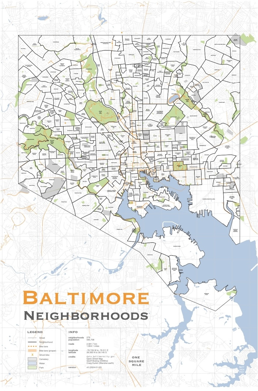
I like this look quite a bit. Lots of other fiddling, including adding cycle lanes in orange (with protected ones even wider), lightening the water and park colors, recoloring the city title, and settling on a format for the legend and the credits, gave me version 4. I added the legend and title manually using PDF Expert’s annotation tools, and then flattened the annotations on export.
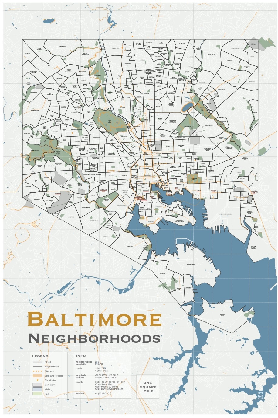
This variant felt a bit too washed out to me, so I darkened the neighborhood boundaries and the water and parks, and then produced version 5, which has a chance of being hung on my wall. There really is no end to the fiddling, and while I have a critical eye, I don’t seem to have the intuitions to guide the design towards something that will please it.
There’s significantly more that could be done to the map. I’m not sure about the reliability of the cycling information on OSM. The city has a nice PDF brochure of city cycle lanes, which has hand-curated routes and is probably more reliable. A next step for me might be to go through the city and manually verify and categorize all the cycling lanes, with the goal of helping produce a more up-to-date map. However, I wonder if some one or group (Bikemore?) has already done this.
If you like, you can download the final map here (PDF, 3.9MB): baltimore-v5-with-legend-flattened.pdf. Is is licensed as CC BY-NC 4.0. I think it looks nice, but I’m afraid I’m too close to it to objectively judge it. If you use it, please let me know!